Requirement 2: Bias in statistical models must be measured and mitigated Requirement 2: Bias in statistical models must be measured and mitigated
There are two widely held misconceptions about bias in statistical prediction systems. The first is that models will only reflect bias if the data they were trained with was itself inaccurate or incomplete. A second is that predictions can be made unbiased by avoiding the use of variables indicating race, gender, or other protected classes.This is known in the algorithmic fairness literature as “fairness through unawareness”; see Moritz Hardt, Eric Price, & Nathan Srebro, Equality of Opportunity in Supervised Learning, Proc. NeurIPS 2016, https://arxiv.org/pdf/1610.02413.pdf, first publishing the term and citing earlier literature for proofs of its ineffectiveness, particularly Pedreshi, Ruggieri, & Turini, Discrimination-aware data mining, Knowledge Discovery & Data Mining, Proc. SIGKDD (2008), http://eprints.adm.unipi.it/2192/1/TR-07-19.pdf.gz. In other fields, blindness is the more common term for the idea of achieving fairness by ignoring protected class variables (e.g., “race-blind admissions” or “gender-blind hiring”). Both of these intuitions are incorrect at the technical level.
It is perhaps counterintuitive, but in complex settings like criminal justice, virtually all statistical predictions will be biased even if the data was accurate, and even if variables such as race are excluded, unless specific steps are taken to measure and mitigate bias. The reason is a problem known as omitted variable bias. Omitted variable bias occurs whenever a model is trained from data that does not include all of the relevant causal factors. Missing causes of the outcome variable that also cause the input variable of interest are known as confounding variables. Moreover, the included variables can be proxies for protected variables like race.Another way of conceiving omitted variable bias is as follows: data-related biases as discussed in Requirement 1 are problems with the rows in a database or spreadsheet: the rows may contain asymmetrical errors, or not be a representative sample of events as they occur in the world. Omitted variable bias, in contrast, is a problem with not having enough or the right columns in a dataset.
Figure 4: Omitted Variable Bias in a Simple Insurance Model
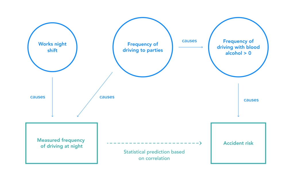
Frequently driving to parties is a confounding variable because it causes both night-time driving and accident risk. A model trained on data about the times of day that drivers drive would exhibit bias against people who work night shifts, because it would conflate the risk of driving to parties with the risk of driving at night.
The diagram also indicates proxy variables at work: frequency of driving at night is a proxy, via driving to parties, for driving while inebriated. It is also a direct proxy for working night shifts. As a result, even though it is not appropriate to charge someone higher insurance premiums simply because they work night shifts, that is the result in this case due to the inclusion of the proxy variable of frequency of driving at night.
Similar networks of proxies apply to criminal risk assessments, from observed input variables such as survey questions asking “How many of your friends/acquaintances have ever been arrested?” or “In your neighborhood, have some of your friends or family been crime victims?” These specific examples are from the Equivant/Northpoint COMPAS risk assessment; see sample questionnaire at https://assets.documentcloud.org/documents/2702103/Sample-Risk-Assessment-COMPAS-CORE.pdf that are proxies for race. As such, it is difficult to separate the use of risk assessment instruments from the use of constitutionally-protected factors such as race to make predictions, and mitigations for this model-level bias are needed.
Methods to Mitigate Bias
Methods to Mitigate Bias
There are numerous possible statistical methods that attempt to correct for bias in risk assessment tools. The correct method to employ will depend on what it means for a tool to be “fair” in a particular application, so this is not only a technical question but also a question of law, policy, and ethics. Although there is not a one-size-fits-all solution to addressing bias, below are some of the possible approaches that might be appropriate in the context of US risk assessment predictions:This list is by no means exhaustive. Another approach involves attempting to de-bias datasets by removing all information regarding the protected class variables. See, e.g., James E. Johndrow & Kristian Lum, An algorithm for removing sensitive information: application to race-independent recidivism prediction, (Mar. 15, 2017), https://arxiv.org/pdf/1703.04957.pdf. Not only would the protected class variable itself be removed but also variation in other variables that is correlated with the protected class variable. This would yield predictions that are independent of the protected class variables, but could have negative implications for accuracy. This method formalizes the notion of fairness known as “demographic parity,” and has the advantage of minimizing disparate impact, such that outcomes should be proportional across demographics. Similar to affirmative action, however, this approach would raise additional fairness questions given different baselines across demographics.
- One approach would be to design the model to satisfy a requirement of “equal opportunity,” meaning that false positive rates (FPRs) are balanced across some set of protected classes (in the recidivism context, the FPR would be the probability that someone who does not recidivate is incorrectly predicted to recidivate).See Moritz Hardt, Eric Price, & Nathan Srebro, Equality of Opportunity in Supervised Learning, Proc. NeurIPS 2016, https://arxiv.org/pdf/1610.02413.pdf. Unequal false positive rates are especially problematic in the criminal justice system since they imply that the individuals who do not recidivate in one demographic group are wrongfully detained at higher rates than non-recidivating individuals in the other demographic group(s). One caveat to this approach is that corrections to ensure protected classes have identical or similar false positive rates will result in differences in overall predictive accuracy between these groups. This is due to different baseline rates of recidivism for different demographic groups in U.S. criminal justice data. See J. Kleinberg, S. Mullainathan, M. Raghavan. Inherent Trade-Offs in the Fair Determination of Risk Scores. Proc. ITCS, (2017), https://arxiv.org/abs/1609.05807 and A. Chouldechova, Fair prediction with disparate impact: A study of bias in recidivism prediction instruments. Proc. FAT/ML 2016, https://arxiv.org/abs/1610.07524. Another caveat is that such a correction can reduce overall utility, as measured as a function of the number of individuals improperly detained or released. See, e.g., Sam Corbett-Davies et al., Algorithmic Decision-Making and the Cost of Fairness, (2017), https://arxiv.org/pdf/1701.08230.pdf. Thus, if an equal opportunity correction is used, then differences in overall accuracy must be evaluated. As long as the training data show higher arrest rates among minorities, statistically accurate scores must of mathematical necessity have a higher false positive rate for minorities. For a paper that outlines how equalizing FPRs (a measure of unfair treatment) requires creating some disparity in predictive accuracy across protected categories, see J. Kleinberg, S. Mullainathan, M. Raghavan. Inherent Trade-Offs in the Fair Determination of Risk Scores. Proc. ITCS, (2017), https://arxiv.org/abs/1609.05807; for arguments about the limitations of FPRs as a sole and sufficient metric, see e.g. Sam Corbett-Davies and Sharad Goel, The Measure and Mismeasure of Fairness: A Critical Review of Fair Machine Learning, working paper, https://arxiv.org/abs/1808.00023.
- A second approach would be to prioritize producing models where the predictive parity of scores is the same across different demographic groups. This property is known as “calibration within groups” and has the benefit of making scores more interpretable across groups. Calibration within groups would entail, for instance, that individuals with a score of 60% have a 60% chance of recidivating, regardless of their demographic group. The issue with this approach is that ensuring predictive parity comes at the expense of the equal opportunity measure described above.Geoff Pleiss et al. On Fairness and Calibration (describing the challenges of using this approach when baselines are different), https://arxiv.org/pdf/1709.02012.pdf. For instance, the COMPAS tool, which is optimized for calibration within groups, has been criticized for its disparate false positive rates. In fact, ProPublica found that even when controlling for prior crimes, future recidivism, age, and gender, black defendants were 77 percent more likely to be assigned higher risk scores than white defendants. The stance that unequal false positive rates represents material unfairness was popularized in a study by Julia Angwin et al. Machine Bias, ProPublica, https://www.propublica.org/article/machine-bias-risk-assessments-in-criminal-sentencing, (2016), and confirmed in further detail in e.g, Julia Dressel and Hany Farid, The accuracy, fairness and limits of predicting recidivism, Science Advances, 4(1), (2018), http://advances.sciencemag.org/content/advances/4/1/eaao5580.full.pdf. Whether or not FPRs are the right measure of fairness is disputed within the statistics literature. This indicates that group-calibrated risk assessment tools may impact non-recidivating individuals differently, depending on their race. See, e.g., Alexandra Chouldechova, Fair prediction with disparate impact: A study of bias in recidivism prediction instruments, Big Data 5(2), https://www.liebertpub.com/doi/full/10.1089/big.2016.0047, (2017).
- A third approach involves using causal inference methods to formalize the permissible and impermissible causal relationships between variables and make predictions using only the permissible pathways. See, e.g., Niki Kilbertus et al., Avoiding Discrimination Through Causal Reasoning, (2018), https://arxiv.org/pdf/1706.02744.pdf. An advantage of this approach is that it formally addresses the difference between correlation and causation and clarifies the causal assumptions underlying the model. It also only removes correlation to the protected class that results from problematic connections between the variables, preserving more information from the data. The shortcoming of this approach is that it requires the toolmaker to have a good understanding of the causal relationships between the relevant variables, so additional subject-matter expertise is necessary to create a valid causal model (Figure 4 shows a simple example in a hypothetical insurance case, but recidivism predictions will likely be far more complex). Moreover, the toolmaker needs to identify which causal relationships are problematic and which are not, Formally, the toolmaker must distinguish “resolved” and “unresolved” discrimination. Unresolved discrimination results from a direct causal path between the protected class and predictor that is not blocked by a “resolving variable.” A resolving variable is one that is influenced by the protected class variable in a manner that we accept as nondiscriminatory. For example, if women are more likely to apply for graduate school in the humanities and men are more likely to apply for graduate school in STEM fields, and if humanities departments have lower acceptance rates, then women might exhibit lower acceptance rates overall even if conditional on department they have higher acceptance rates. In this case, the department variable can be considered a resolving variable if our main concern is discriminatory admissions practices. See, e.g., Niki Kilbertus et al., Avoiding Discrimination Through Causal Reasoning, (2018), https://arxiv.org/pdf/1706.02744.pdf. so validity further depends on the toolmaker exercising proper judgment.
Given that some of these approaches are in tension with each other, it is not possible to simultaneously optimize for all of them. Nonetheless, these approaches can highlight relevant fairness issues to consider in evaluating tools. For example, even though it is generally not possible to simultaneously satisfy calibration within groups and equal opportunity (Methods #1 and #2 above) with criminal justice data, it would be reasonable to avoid using tools that either have extremely disparate predictive parity across demographics (i.e., poor calibration within groups) or extremely disparate false positive rates across demographics (i.e., low equal opportunity).
Given that each of these approaches involves inherent trade-offs,In addition to the trade-offs highlighted in this section, it should be noted that these methods require a precise taxonomy of protected classes. Although it is common in the United States to use simple taxonomies defined by the Office of Management and Budget (OMB) and the US Census Bureau, such taxonomies cannot capture the complex reality of race and ethnicity. See Revisions to the Standards for the Classification of Federal Data on Race and Ethnicity, 62 Fed. Reg. 210 (Oct 1997), https://www.govinfo.gov/content/pkg/FR-1997-10-30/pdf/97-28653.pdf. Nonetheless, algorithms for bias correction have been proposed that detect groups of decision subjects with similar circumstances automatically. For an example of such an algorithm, see Tatsunori Hashimoto et al., Fairness Without Demographics in Repeated Loss Minimization, Proc. ICML 2018, http://proceedings.mlr.press/v80/hashimoto18a/hashimoto18a.pdf. Algorithms have also been developed to detect groups of people that are spatially or socially segregated. See, e.g., Sebastian Benthall & Bruce D. Haynes, Racial categories in machine learning, Proc. FAT* 2019, https://dl.acm.org/authorize.cfm?key=N675470. Further experimentation with these methods is warranted. For one evaluation, see Jon Kleinberg, An Impossibility Theorem for Clustering, Advances in Neural Information Processing Systems 15, NeurIPS 2002. it is also reasonable to use a few different methods and compare the results between them. This would yield a range of predictions that could better inform decision-making. The best way to do this deserves further research on human-computer interaction. For instance, if judges are shown multiple predictions labelled “zero disparate impact for those who will not reoffend”, “most accurate prediction,” “demographic parity,” etc, will they understand and respond appropriately? If not, decisions about what bias corrections to use might be better made at the level of policymakers or technical government experts evaluating these tools. In addition, appropriate paths for consideration include relying on timely, properly resourced, individualized hearings rather than machine learning tools, developing cost-benefit analyses that place explicit value on avoiding disparate impact, Cost benefit models require explicit tradeoff choices to be made between different objectives including liberty, safety, and fair treatment of different categories of defendants. These choices should be explicit, and must be made transparently and accountably by policymakers. For a macroscopic example of such a calculation see David Roodman, The Impacts of Incarceration on Crime, Open Philanthropy Project report, September 2017, p p131, at https://www.openphilanthropy.org/files/Focus_Areas/Criminal_Justice_Reform/The_impacts_of_incarceration_on_crime_10.pdf. or delaying tool deployment until further columns of high quality data can be collected to facilitate more-accurate and less-biased predictions.